import EoN
import networkx as nx
import matplotlib.pyplot as plt
import random
import scipy
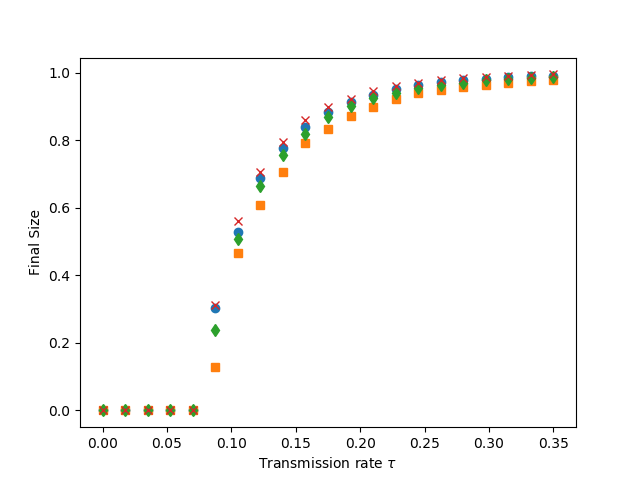
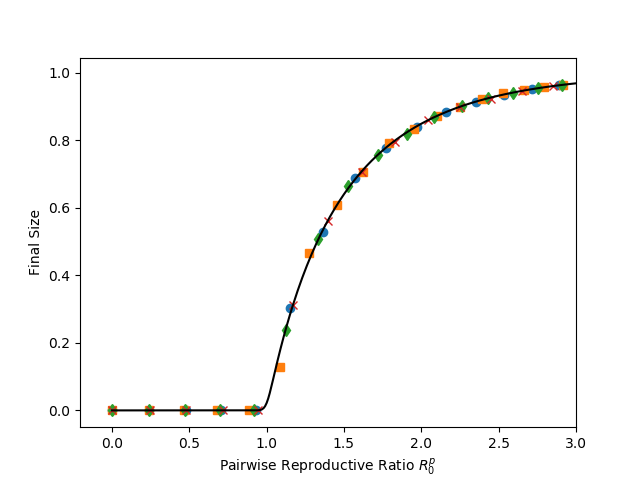
print("for figure 9.5, we have not coded up the equations to calculate size as a function of tau (fig a), so this just gives simulations. It does calculate the predicted size as a function of R_0^p. (fig b)")
r'''
Rather than doing the dynamic simulations, this uses the directed percolation approach
described in chapter 6.
'''
N = 100000
gamma = 1./5.5
tau = 0.55
iterations = 1
rho = 0.001
kave=15
def rec_time_fxn_gamma(u, alpha, beta):
return scipy.random.gamma(alpha,beta)
def rec_time_fxn_fixed(u):
return 1
def rec_time_fxn_exp(u):
return random.expovariate(1)
def trans_time_fxn(u, v, tau):
if tau >0:
return random.expovariate(tau)
else:
return float('Inf')
def R0first(tau):
return (kave-1) * (1- 4/(2+tau)**2)
def R0second(tau):
return (kave-1) * (1- 1/scipy.sqrt(1+2*tau))
def R0third(tau):
return (kave-1)*tau/(tau+1)
def R0fourth(tau):
return (kave-1)*(1-scipy.exp(-tau))
G = nx.configuration_model([kave]*N)
taus = scipy.linspace(0,0.35,21)
def do_calcs_and_plot(G, trans_time_fxn, rec_time_fxn, trans_time_args, rec_time_args, R0fxn, symbol):
As = []
for tau in taus:
P, A = EoN.estimate_nonMarkov_SIR_prob_size_with_timing(G,trans_time_fxn=trans_time_fxn,
rec_time_fxn = rec_time_fxn,
trans_time_args = (tau,),
rec_time_args=rec_time_args)
As.append(A)
plt.figure(1)
plt.plot(taus, As, symbol)
plt.figure(2)
plt.plot( R0fxn(taus), As, symbol)
print("first distribution")
do_calcs_and_plot(G, trans_time_fxn, rec_time_fxn_gamma, (tau,), (2,0.5), R0first, 'o')
print("second distribution")
do_calcs_and_plot(G, trans_time_fxn, rec_time_fxn_gamma, (tau,), (0.5,2), R0second, 's')
print("fourth distribution")
do_calcs_and_plot(G, trans_time_fxn, rec_time_fxn_exp, (tau,), (), R0third, 'd')
print("fifth distribution")
do_calcs_and_plot(G, trans_time_fxn, rec_time_fxn_fixed, (tau,), (), R0fourth, 'x')
plt.figure(1)
plt.xlabel(r'Transmission rate $\tau$')
plt.ylabel('Final Size')
plt.savefig('fig9p5a.png')
R0s = scipy.linspace(0,3,301)
ps = R0s/(kave-1)
Apred = [EoN.Attack_rate_discrete({kave:1}, p) for p in ps]
plt.figure(2)
plt.plot(R0s, Apred, '-', color = 'k')
plt.axis(xmax = 3)
plt.xlabel('Pairwise Reproductive Ratio $R_0^p$')
plt.ylabel('Final Size')
plt.savefig('fig9p5b.png')