import EoN
import networkx as nx
import matplotlib.pyplot as plt
import random
import scipy
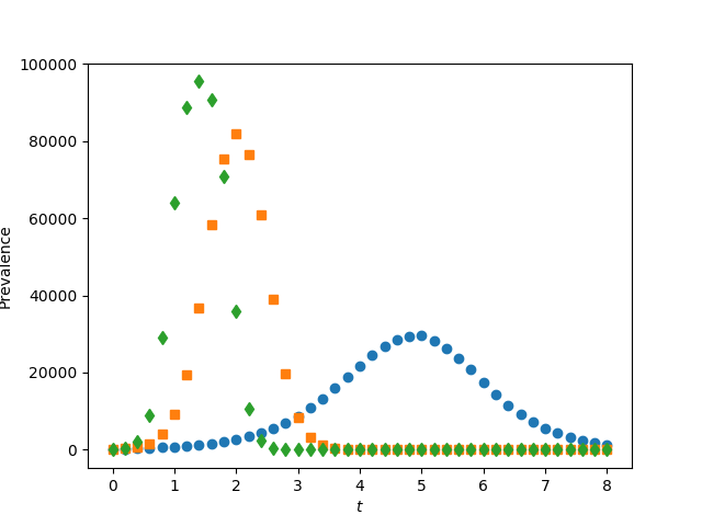
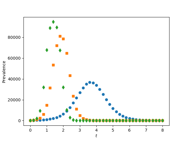
print("for figure 9.4, we have not yet coded up the system of equations, so this just gives simulations")
r'''We use a large value of N and only a single iteration. The code is
similar to fig 9.2's code, but the loops are structured a little differently.
We loop over graph type first.
then we loop over kave.
'''
N = 100000
n = 10
gamma = 1./5.5
tau = 0.55
iterations = 1
rho = 0.001
def rec_time_fxn(u):
return 1
def trans_time_fxn(u, v, tau):
return random.expovariate(tau)
def ER_graph_generation(N, kave):
return nx.fast_gnp_random_graph(N, kave/(N-1.))
def regular_graph_generation(N, kave):
return nx.configuration_model([kave]*N)
display_ts = scipy.linspace(0, 8, 41) #[0, 0.2, 0.4, ..., 7.8, 8]
for graph_algorithm, filename in ([regular_graph_generation, 'fig9p4a.png'], [ER_graph_generation, 'fig9p4b.png']):
plt.clf()
for kave, symbol in ([5, 'o'], [10, 's'], [15, 'd']):
print(kave)
G = graph_algorithm(N, kave)
t, S, I, R = EoN.fast_nonMarkov_SIR(G,
trans_time_fxn=trans_time_fxn,
trans_time_args=(tau,),
rec_time_fxn=rec_time_fxn,
rec_time_args=(),
rho=rho)
newI = EoN.subsample(display_ts, t, I)
plt.plot(display_ts, newI, symbol)
plt.xlabel('$t$')
plt.ylabel('Prevalence')
plt.savefig(filename)