Figure 9.2 (a and b)

Downloadable Source Code

import EoN
import networkx as nx
import matplotlib.pyplot as plt
import random
import scipy

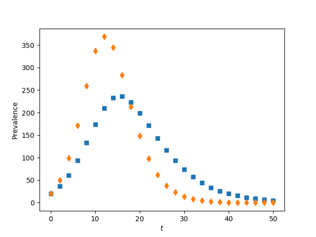
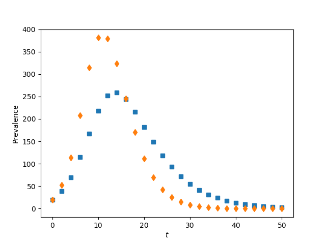
print("for figure 9.2, we have not yet coded up the system of equations (9.5), so this just gives simulations")
N = 1000
n = 10
gamma = 1./5.5
tau = 0.545/n
iterations = 250
rho = 0.02

ER = nx.fast_gnp_random_graph(N, n/(N-1.)) #erdos-renyi graph
regular = nx.configuration_model([n]*N) # [n]*N is [n,n, ..., n]

def rec_time_fxn(u, K, gamma):
    duration = 0
    for counter in range(K):
        duration += random.expovariate(K*gamma)
    return duration

def trans_time_fxn(u, v, tau):
    return random.expovariate(tau)

display_ts = scipy.linspace(0, 50, 26)
for G, filename in ([regular, 'fig9p2a.png'], [ER, 'fig9p2b.png']):
    plt.clf()
    Isum = scipy.zeros(len(display_ts))
    for K, symbol in ([1, 's'], [3, 'd']):
        for counter in range(iterations):
            t, S, I, R = EoN.fast_nonMarkov_SIR(G,
                                                trans_time_fxn=trans_time_fxn,
                                                trans_time_args=(tau,),
                                                rec_time_fxn=rec_time_fxn,
                                                rec_time_args=(K, gamma),
                                                rho=rho)
            newI = EoN.subsample(display_ts, t, I)
            Isum += newI
        Isum /= iterations
        plt.plot(display_ts, Isum, symbol)
    plt.xlabel('$t$')
    plt.ylabel('Prevalence')
    plt.savefig(filename)