Figure 5.2 (a, b, c, and d)

• Note that the book has a typo. As with fig 4.7, for (c), $\tau = 1.1\tau_c$.
• It’s worth looking at $1.2\tau_c$ as well. It’s interesting.

Downloadable Source Code

import EoN
import networkx as nx
import matplotlib.pyplot as plt
import scipy



N=100000  #100 times as large as the value given in the text
gamma = 1.
iterations = 1
rho = 0.05
tmax = 20
tcount = 1001
kave = 20.
ksqave = (5**2 + 35**2)/2.

tau_c = gamma*kave/ksqave

ksmall = 5
kbig = 35
deg_dist = [ksmall, kbig]*int(N/2)

report_times = scipy.linspace(0, tmax, tcount)

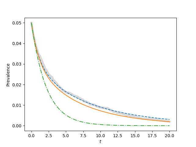
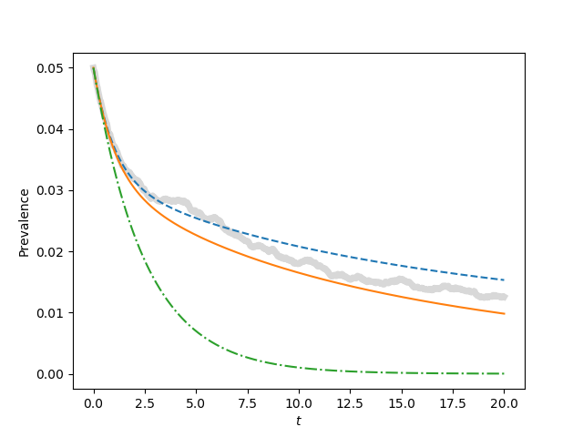
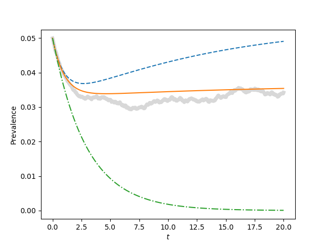
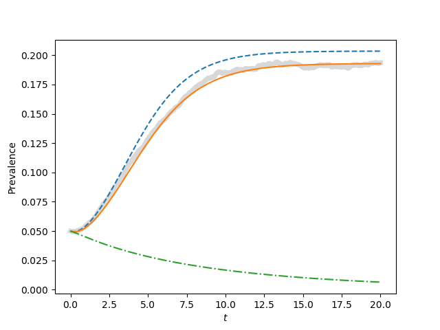
for tau, label in zip([0.9*tau_c, tau_c, 1.1*tau_c, 1.5*tau_c],['a', 'b', 'c', 'd']):
    print(str(tau_c)+" "+str(tau))
    plt.clf()

    Isum = scipy.zeros(tcount)
    for counter in range(iterations):
        G = nx.configuration_model(deg_dist)
        t, S, I = EoN.fast_SIS(G, tau, gamma, tmax=tmax, rho=rho)
        I = I*1./N
        I = EoN.subsample(report_times, t, I)
        Isum += I
    plt.plot(report_times, Isum/iterations, color='grey', linewidth=5, alpha=0.3)

    degree_array = scipy.zeros(kbig+1)
    degree_array[kbig]=N/2
    degree_array[ksmall]=N/2
    Sk0 = degree_array*(1-rho)
    Ik0 = degree_array*rho

    t, S, I = EoN.SIS_heterogeneous_meanfield(Sk0, Ik0, tau, gamma, tmax=tmax,
                                                tcount=tcount)
    plt.plot(t, I/N, '--')


    SI0 = ((kbig + ksmall)*N/2.)*(1-rho)*rho
    SS0 = ((kbig+ksmall)*N/2.)*(1-rho)*(1-rho)
    II0 = ((kbig+ksmall)*N/2.)*rho*rho

    t, S, I = EoN.SIS_compact_pairwise(Sk0, Ik0, SI0, SS0, II0, tau, gamma,
                                tmax=tmax, tcount=tcount)
    plt.plot(t, I/N)
    #t, S, I = EoN.SIS_compact_pairwise(Sk0, I0, SI0, SS0, II0, tau, gamma, tmax=tmax, tcount=tcount)
    #plt.plot(t, I/N)

    I0 = N*rho
    S0 = N*(1-rho)
    kave = (kbig+ksmall)/2.

    t, S, I = EoN.SIS_homogeneous_pairwise(S0, I0, SI0, SS0, kave, tau, gamma, tmax=tmax, tcount=tcount)
    plt.plot(t, I/N, '-.')
    plt.xlabel('$t$')
    plt.ylabel('Prevalence')
    plt.savefig('fig5p2{}.png'.format(label))