Figure 4.13

Downloadable Source Code

import EoN
import networkx as nx
import matplotlib.pyplot as plt
import scipy

r'''
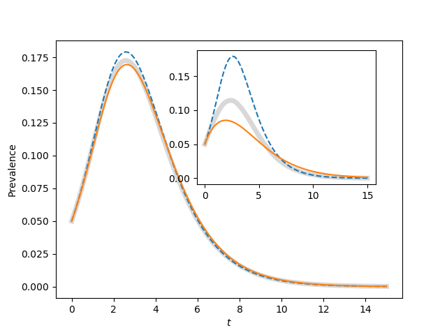
Reproduces figure 4.13

With N=1000, there is still significant stochasticity.  Some epidemics have earlier
peaks than others.  When many of these are averaged together, the final outcome
is that the average has a lower, broader peak than a typical epidemic.  In
this case it tends to make the Erdos-Renyi network for <K>=50 look like a better
fit for the homogeneous_pairwise model.

Increasing N to 10000 will eliminate this.
'''

print("Often stochastic effects cause the peak for <K>=50 to be lower than predicted.")
print("See comments in code for explanation")



N=10000
gamma = 1.
iterations = 200
rho = 0.05
tmax = 15
tcount = 1001

report_times = scipy.linspace(0,tmax,tcount)
ax1 = plt.gca()#axes([0.1,0.1,0.9,0.9])
ax2 = plt.axes([0.44,0.45,0.4,0.4])

for kave, ax in zip((50, 5), (ax1, ax2)):
    tau = 2*gamma/kave
    Isum = scipy.zeros(tcount)

    for counter in range(iterations):
        G = nx.fast_gnp_random_graph(N,kave/(N-1.))
        t, S, I, R = EoN.fast_SIR(G, tau, gamma, tmax=tmax, rho=rho)
        I = I*1./N
        I = EoN.subsample(report_times, t, I)
        Isum += I
    ax.plot(report_times, Isum/iterations, color='grey', linewidth=5, alpha=0.3)

    S0 = (1-rho)*N
    I0 = rho*N
    R0=0

    t, S, I, R = EoN.SIR_homogeneous_meanfield(S0, I0, R0, kave, tau, gamma,
                                            tmax=tmax, tcount=tcount)
    ax.plot(t, I/N, '--')

    SI0 = (1-rho)*N*kave*rho
    SS0 = (1-rho)*N*kave*(1-rho)
    t, S, I, R = EoN.SIR_homogeneous_pairwise(S0, I0, R0, SI0, SS0, kave, tau, gamma,
                                tmax=tmax, tcount=tcount)
    ax.plot(t, I/N)


ax1.set_xlabel('$t$')
ax1.set_ylabel('Prevalence')
plt.savefig('fig4p13.png')