Figure 1.2

Downloadable Source Code

import EoN
import networkx as nx
from matplotlib import rc
import matplotlib.pylab as plt


import scipy
import random



colors = ['#5AB3E6','#FF2000','#009A80','#E69A00', '#CD9AB3', '#0073B3',
        '#F0E442']

#commands to make legend be in LaTeX font
#rc('font', **{'family': 'serif', 'serif': ['Computer Modern']})
rc('text', usetex=True)



rho = 0.025
target_k = 6
N=10000
tau = 0.5
gamma = 1.
ts = scipy.arange(0,40,0.05)
count = 50 #number of simulations to run for each



def generate_network(Pk, N, ntries = 100):
    r'''Generates an N-node random network whose degree distribution is given by Pk'''
    counter = 0
    while counter< ntries:
        counter += 1
        ks = []
        for ctr in range(N):
            ks.append(Pk())
        if sum(ks)%2 == 0:
            break
    if sum(ks)%2 ==1:
        raise EoN.EoNError("cannot generate even degree sum")
    G = nx.configuration_model(ks)
    return G



#An erdos-renyi network has a Poisson degree distribution.
def PkPoisson():
    return scipy.random.poisson(target_k)
def PsiPoisson(x):
    return scipy.exp(-target_k*(1-x))
def DPsiPoisson(x):
    return target_k*scipy.exp(-target_k*(1-x))



#a regular (homogeneous) network has a simple generating function.

def PkHomogeneous():
    return target_k
def PsiHomogeneous(x):
    return x**target_k
def DPsiHomogeneous(x):
    return target_k*x**(target_k-1)




#The following 30 - 40 lines or so are devoted to defining the degree distribution
#and the generating function of the truncated power law network.

#defining the power law degree distribution here:
assert(target_k==6) #if you've changed target_k, then you'll
                #want to update the range 1..61 and/or
                #the exponent 1.5.

PlPk = {}
exponent = 1.5
kave = 0
for k in range(1,61):
    PlPk[k]=k**(-exponent)
    kave += k*PlPk[k]

normfactor= sum(PlPk.values())
for k in PlPk:
    PlPk[k] /= normfactor

def PkPowLaw():
    r = random.random()
    for k in PlPk:
        r -= PlPk[k]
        if r<0:
            return k

def PsiPowLaw(x):
    #print PlPk
    rval = 0
    for k in PlPk:
        rval += PlPk[k]*x**k
    return rval

def DPsiPowLaw(x):
    rval = 0
    for k in PlPk:
        rval += k*PlPk[k]*x**(k-1)
    return rval
#End of power law network properties.





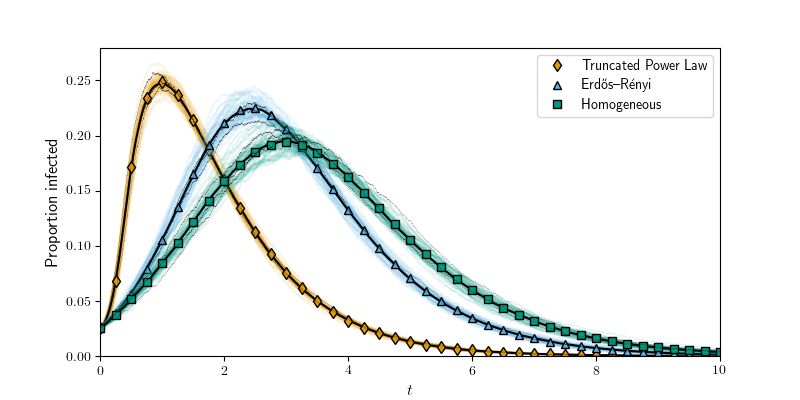
def process_degree_distribution(N, Pk, color, Psi, DPsi, symbol, label, count):
    report_times = scipy.linspace(0,30,3000)
    sums = 0*report_times
    for cnt in range(count):
        G = generate_network(Pk, N)
        t, S, I, R = EoN.fast_SIR(G, tau, gamma, rho=rho)
        plt.plot(t, I*1./N, '-', color = color,
                                alpha = 0.1, linewidth=1)
        subsampled_I = EoN.subsample(report_times, t, I)
        sums += subsampled_I*1./N
    ave = sums/count
    plt.plot(report_times, ave, color = 'k')

    #Do EBCM
    N= G.order()#N is arbitrary, but included because our implementation of EBCM assumes N is given.
    t, S, I, R = EoN.EBCM_uniform_introduction(N, Psi, DPsi, tau, gamma, rho, tmin=0, tmax=10, tcount = 41)
    plt.plot(t, I/N, symbol, color = color, markeredgecolor='k', label=label)

    for cnt in range(3):  #do 3 highlighted simulations
        G = generate_network(Pk, N)
        t, S, I, R = EoN.fast_SIR(G, tau, gamma, rho=rho)
        plt.plot(t, I*1./N, '-', color = 'k', linewidth=0.1)




plt.figure(figsize=(8,4))



#Powerlaw
process_degree_distribution(N, PkPowLaw, colors[3], PsiPowLaw, DPsiPowLaw, 'd', r'Truncated Power Law', count)

#Poisson
process_degree_distribution(N, PkPoisson, colors[0], PsiPoisson, DPsiPoisson, '^', r'Erd\H{o}s--R\'{e}nyi', count)

#Homogeneous
process_degree_distribution(N, PkHomogeneous, colors[2], PsiHomogeneous, DPsiHomogeneous, 's', r'Homogeneous', count)

plt.xlabel(r'$t$', fontsize=12)
plt.ylabel(r'Proportion infected', fontsize=12)
plt.legend(loc = 'upper right', numpoints = 1)

plt.axis(xmax=10, xmin=0, ymin=0)
plt.savefig('fig1p2.pdf')