import EoN
import networkx as nx
import random
import matplotlib.pyplot as plt
G= nx.bipartite.configuration_model([1,11]*2000, [3]*8000)
#the graph now consists of two parts. The first part has 2000 degree 1 nodes
#and 2000 degree 11 nodes. The second has 8000 degree 3 nodes.
#there are 24000 edges in the network.
#
# We assume the first ones are twice as infectious as the second ones.
#
for node in G:
if G.degree(node) in [1,11]:
G.node[node]['type'] = 'A'
else:
G.node[node]['type'] = 'B'
#We have defined the two types of nodes.
#now define the transmission and recovery functions:
def trans_time_function(source, target, tau):
if G.node[source]['type'] is 'A':
return random.expovariate(2*tau)
else:
return random.expovariate(tau)
def rec_time_function(node, gamma):
return random.expovariate(gamma)
tau = 0.4
gamma = 1.
sim = EoN.fast_nonMarkov_SIR(G, trans_time_function, rec_time_function,
trans_time_args=(tau,), rec_time_args=(gamma,),
rho = 0.01, return_full_data=True)
t, S, I, R = sim.summary()
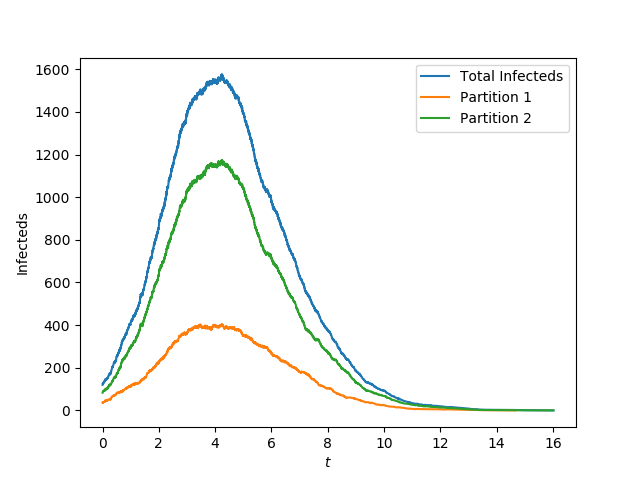
plt.plot(t, I, label='Total Infecteds')
t1, S1, I1, R1 = sim.summary(nodelist = [node for node in G if G.node[node]['type']=='A'])
plt.plot(t1, I1, label = 'Partition 1')
t2, S2, I2, R2 = sim.summary(nodelist = [node for node in G if G.node[node]['type']=='B'])
plt.plot(t2, I2, label = 'Partition 2')
plt.legend()
plt.xlabel('$t$')
plt.ylabel('Infecteds')
plt.savefig('bipartite.png')