SIRV display and animation example

Downloadable Source Code

The code below looks at an SIRV epidemic (SIR + vaccination) and produces the image

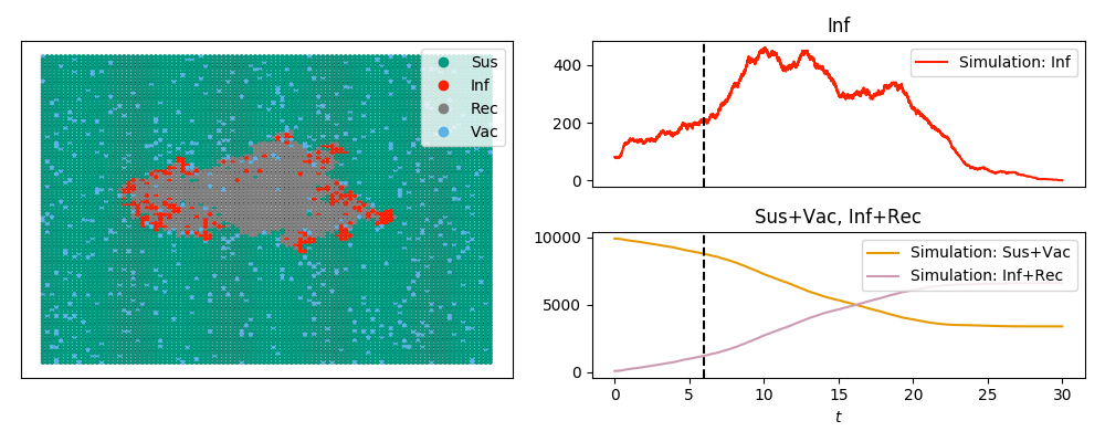
and the animation

Note that the labels are in plain text rather than math mode (since tex=False). Note also that we can plot 'Sus'+'Vac' and similar time series using the commands here.

If we use a model with other states than 'S', 'I', and 'R', the default colors aren’t specified. In this case we need to do a little bit more.

Consider a model where the states are 'Sus', 'Inf', 'Rec', or 'Vac'. That is, an SIR model with vaccination. We will use Gillespie_simple_contagion for this. I’m choosing the status names to be longer than one character to show changes in the argument ts_plots stating what the time-series plots should show.

In this model, susceptible people have a rate of becoming vaccinated which is independent of the disease status. Otherwise, it is just like the SIR disease in the previous example. So the “spontaneous transitions” are 'Suc' to 'Vac' with rate 0.01 and 'Inf' to 'Rec' with rate 1.0. The “induced transitions” are ('Inf', 'Sus') to ('Inf', 'Inf') with rate 2.0.

The method is built on Gillespie_simple_contagion

import networkx as nx
import EoN
import matplotlib.pyplot as plt
from collections import defaultdict

G = nx.grid_2d_graph(100,100) #each node is (u,v) where 0<=u,v<=99
#we'll initially infect those near the middle
initial_infections = [(u,v) for (u,v) in G if 45<u<55 and 45<v<55]

H = nx.DiGraph()  #the spontaneous transitions
H.add_edge('Sus', 'Vac', rate = 0.01)
H.add_edge('Inf', 'Rec', rate = 1.0)

J = nx.DiGraph()  #the induced transitions
J.add_edge(('Inf', 'Sus'), ('Inf', 'Inf'), rate = 2.0)

IC = defaultdict(lambda:'Sus')
for node in initial_infections:
    IC[node] = 'Inf'

return_statuses = ['Sus', 'Inf', 'Rec', 'Vac']

color_dict = {'Sus': '#009a80','Inf':'#ff2000', 'Rec':'gray','Vac': '#5AB3E6'}
pos = {node:node for node in G}
tex = False
sim_kwargs = {'color_dict':color_dict, 'pos':pos, 'tex':tex}

sim = EoN.Gillespie_simple_contagion(G, H, J, IC, return_statuses, tmax=30, return_full_data=True, sim_kwargs=sim_kwargs)

times, D = sim.summary()
#
#imes is a numpy array of times.  D is a dict, whose keys are the entries in
#return_statuses.  The values are numpy arrays giving the number in that
#status at the corresponding time.

newD = {'Sus+Vac':D['Sus']+D['Vac'], 'Inf+Rec' : D['Inf'] + D['Rec']}
#
#newD is a new dict giving number not yet infected or the number ever infected
#Let's add this timeseries to the simulation.
#
new_timeseries = (times, newD)
sim.add_timeseries(new_timeseries, label = 'Simulation', color_dict={'Sus+Vac':'#E69A00', 'Inf+Rec':'#CD9AB3'})

sim.display(6, node_size = 4, ts_plots=[['Inf'], ['Sus+Vac', 'Inf+Rec']])
plt.savefig('SIRV_display.png')

ani=sim.animate(ts_plots=[['Inf'], ['Sus+Vac', 'Inf+Rec']], node_size = 4)
ani.save('SIRV_animate.mp4', fps=5, extra_args=['-vcodec', 'libx264'])