Getting Started

Installation

You can install EoN version 1.1 with pip

pip install EoN

If you have installed a previous version and want to reinstall the most recent version available through pip (1.1). The easiest way is

pip uninstall EoN
pip install EoN

To install EoN a later (in development) version You can clone or download the Github version at https://github.com/springer-math/Mathematics-of-Epidemics-on-Networks

Then just move into the main directory and run

python setup.py install

The documentation provided here is for version 1.1.

If you want to see changes from previous versions, please see Changes from v1.0.

If you use EoN, or publish anything based on it, please cite the Journal of Open Source Software publication

Also, please let me know so that I can use it for performance reviews and grant applications and generally because it makes me happy.

QuickStart Guide

The code here provides an example of creating a Barabasi-Albert network. Then it performs several simulations of an SIR epidemic starting with a fraction rho randomly infected initially. Finally it uses several analytic models to predict the spread of an epidemic in a random network with the given properties.

import networkx as nx
import matplotlib.pyplot as plt
import EoN

N=10**5
G=nx.barabasi_albert_graph(N, 5) #create a barabasi-albert graph

tmax = 20
iterations = 5  #run 5 simulations
tau = 0.1           #transmission rate
gamma = 1.0    #recovery rate
rho = 0.005      #random fraction initially infected

for counter in range(iterations): #run simulations
    t, S, I, R = EoN.fast_SIR(G, tau, gamma, rho=rho, tmax = tmax)
    if counter == 0:
        plt.plot(t, I, color = 'k', alpha=0.3, label='Simulation')
    plt.plot(t, I, color = 'k', alpha=0.3)

#Now compare with ODE predictions.  Read in the degree distribution of G
#and use rho to initialize the various model equations.
#There are versions of these functions that allow you to specify the
#initial conditions rather than starting from a graph.

#we expect a homogeneous model to perform poorly because the degree
#distribution is very heterogeneous
t, S, I, R = EoN.SIR_homogeneous_pairwise_from_graph(G, tau, gamma, rho=rho, tmax = tmax)
plt.plot(t, I, '-.', label = 'Homogeneous pairwise', linewidth = 5)

#meanfield models will generally overestimate SIR growth because they
#treat partnerships as constantly changing.
t, S, I, R = EoN.SIR_heterogeneous_meanfield_from_graph(G, tau, gamma, rho=rho, tmax=tmax)
plt.plot(t, I, ':', label = 'Heterogeneous meanfield', linewidth = 5)

#The EBCM model does not account for degree correlations or clustering
t, S, I, R = EoN.EBCM_from_graph(G, tau, gamma, rho=rho, tmax = tmax)
plt.plot(t, I, '--', label = 'EBCM approximation', linewidth = 5)

#the preferential mixing model captures degree correlations.
t, S, I, R = EoN.EBCM_pref_mix_from_graph(G, tau, gamma, rho=rho, tmax=tmax)
plt.plot(t, I, label = 'Pref mix EBCM', linewidth=5, dashes=[4, 2, 1, 2, 1, 2])

plt.xlabel('$t$')
plt.ylabel('Number infected')

plt.legend()
plt.savefig('SIR_BA_model_vs_sim.png')

This produces

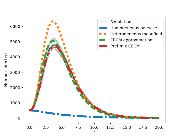
The preferential mixing version of the EBCM approach provides the best approximation to the (gray) simulated epidemics. We now move on to SIS epidemics:

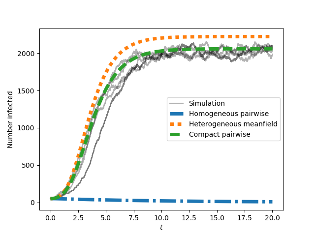
plt.clf()

#Now run for SIS.   Simulation is much slower so need smaller network
N=10**4
G=nx.barabasi_albert_graph(N, 5) #create a barabasi-albert graph
for counter in range(iterations):
    t, S, I = EoN.fast_SIS(G, tau, gamma, rho=rho, tmax = tmax)
    if counter == 0:
        plt.plot(t, I, color = 'k', alpha=0.3, label='Simulation')
    plt.plot(t, I, color = 'k', alpha=0.3)

#Now compare with ODE predictions.  Read in the degree distribution of G
#and use rho to initialize the various model equations.
#There are versions of these functions that allow you to specify the
#initial conditions rather than starting from a graph.

#we expect a homogeneous model to perform poorly because the degree
#distribution is very heterogeneous
t, S, I = EoN.SIS_homogeneous_pairwise_from_graph(G, tau, gamma, rho=rho, tmax = tmax)
plt.plot(t, I, '-.', label = 'Homogeneous pairwise', linewidth = 5)

t, S, I = EoN.SIS_heterogeneous_meanfield_from_graph(G, tau, gamma, rho=rho, tmax=tmax)
plt.plot(t, I, ':', label = 'Heterogeneous meanfield', linewidth = 5)

t, S, I = EoN.SIS_compact_pairwise_from_graph(G, tau, gamma, rho=rho, tmax=tmax)
plt.plot(t, I, '--', label = 'Compact pairwise', linewidth = 5)

plt.xlabel('$t$')
plt.ylabel('Number infected')
plt.legend()
plt.savefig('SIS_BA_model_vs_sim.png')

This produces